As data analysts, we all try to do the right thing. When there is a choice of statistical distributions to be used for a given application, it’s a natural inclination to try to find the “best” one.
But beware...
Fishing for the best distribution can lead you into a trap. Just because one option appears to be best – that doesn’t mean that it’s correct! For example, consider this data set:
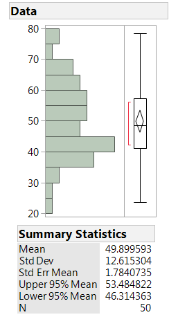 What is the best distribution we can use to describe this data? JMP can help us answer this question. From the Distribution platform, we can choose to fit a number of common distributions to the data: Normal, Weibull, Gamma, Exponential, and others. To fit all possible continuous distributions to this data in JMP, go to the red triangle hotspot for this variable in the Distribution report, and choose “Continuous Fit > All”. Here is the result:
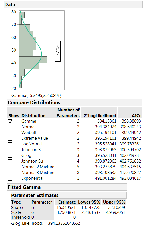 JMP has compared 11 potential distributions for this data, and ranked them from best (Gamma) to worst (Exponential). The metric used to perform the ranking is the corrected Akaike Information Criterion (AICc). Lower values of AICc indicate better fit, and so the Gamma distribution is the winner here.
Here’s the catch
This data set was generated by drawing a random sample of size 50 from a population that is normally distributed with a mean of 50 and a standard deviation of 10. The Normal distribution is the correct answer by definition, but our fishing expedition gave us a misleading result.
How often is there a mismatch like this? One way we can approach this question is through simulation. I wrote a small JMP script to draw samples of various sizes from a normally distributed population. I investigated sample sizes of 5, 10, 20, 30, 50, 75, 100, 250, and 500 observations; for each of these, I drew 1,000 independent samples and had JMP compute the fit for all possible continuous distributions. Last, for each sample I recorded the name of the best-fitting distribution, as measured by AICc. (JSL script available in the JMP File Exchange).
The results were quite surprising!
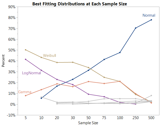
- Remember, the correct answer in each case is “Normal”. If our fishing expedition was yielding good results across the board, the line for the Normal distribution should be high and flat, hovering near 100%.
- Instead, the wrong distribution was chosen with disturbing frequency. For sample sizes under 50, the Normal distribution was not even the most commonly chosen. That honor belongs to the Weibull distribution.
- For a sample size of 5 observations from a Normal distribution, the correct identification was not made a single time out of 1,000 samples.
- If you want to have at least a 50% chance of correctly identifying normally distributed data by this method, you’ll need more than 100 observations!
- Even at a sample size of 500 observations, the likelihood of the normal distribution being correctly called the best is only about 80%.
The moral of the story
When comparing the fit of different distributions to a data set, don’t assume that the distribution with the smallest AICc is the correct one. Relative magnitudes of the AICc statistics are what counts. A rule of thumb (used elsewhere in JMP) is that models whose values of AICc are within 10 units of the “best” one are roughly equivalent.* In our first example above, the Gamma distribution is nominally the best, but its AICc is only .2 units lower than that of the Normal distribution. There is not good statistical evidence to choose the Gamma over the Normal.
More generally, as a best practice it is wise to consider only distributions that make sense in the context of the problem. Your own knowledge and expertise are usually the best guides. Don’t choose an exotic distribution that has a slightly better fit over one that makes sense and has a proven track record in your field of work.
*This rule is used to compare models built in the Generalized Regression personality of the Fit Model platform in JMP Pro. See Burnham, K.P. and Anderson, D.R. (2002), Model Selection And Multimodel Inference: A Practical Information Theoretic Approach. Springer, New York.

