For college football, the regular season is coming to an end, and in a few days we’ll know which teams are going to which end-of-season bowl games. Though some bowl assignments are determined by formula, each bowl often has a choice of several teams to invite to their game. Some teams have a reputation for “traveling well,” meaning they have a fan base that can raise attendance for far away games or for drawing a large TV audience. For instance, consider this blog post comment regarding Ohio State:
Buckeye Nation traveling well is an understatement. We are the best traveling college football fans in the nation.
I wondered if the numbers support the reputations and set out to collect attendance and TV ratings data. I put together 11 years of bowl games data, mostly from bcsfootball.org with some holes filled in from individual bowl Web sites. As often is the case, cleaning the data was a major undertaking. I used the Recode feature in JMP to standardize team names (“Connecticut” or “UConn”) and bowl names. Bowl names are particularly tricky as the actual names sometimes change over the years, and sometimes the same name has been used for different bowls (“Meineke Car Care Bowl” is one example). I used the JMP Geocoder add-in to determine locations to compute travel distances.
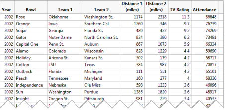
More variables would surely be helpful, though I’m hoping that the bowl itself serves as a proxy for variables like team ranking (since each bowl sits in a fairly stable slot in the bowl pecking order). Looking at models that include Year, Bowl, Year * Bowl, Team and Distance, it turns out that attendance and TV ratings behave quite differently. Almost all of the Bowl and Year * Bowl interactions are strongly correlated with Attendance, but only a few of them are correlated with TV Rating. Apparently, TV ratings are more likely influenced by which teams are playing. Distance is a relatively weak factor overall, and there’s not enough data to see how it applies to individual teams.
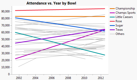
Bowl attendance trends vary by bowl, with some bowls being stable, some trending up and some trending down. The following graph shows the trends lines, with two from each category highlighted.
Turning to the teams, a complication with this data is that there are two Team columns and thus two team values per row. Stacking the team columns is possible, but it results in duplicate bowl-year rows (artificially reducing their p-values) and more importantly disassociates the two opposing teams so we can no longer model the shared responsibility for the results. A better approach is to create indicator columns, one per team, such that exactly two of the columns would be non-zero for each game. I found Table > Summary with Team as a subgroup to be a convenient way to generate the indicator columns.
Including the indicator columns with the Year and Bowl columns lets us see the effect of each team after accounting for the effect of the Year and Bowl. As I mentioned above, attendance is modeled very well by the combination of those two variables, and perhaps for that reason there are few teams with significant model effects. Here are those with the smallest p-values, sorted by the estimate value. Hawaii is a special circumstance since that school often plays in the Hawaii Bowl, and in general the Hawaii Bowl attendance is much higher when Hawaii plays in it.
|
| Term |
|---|
| Estimate |
|---|
| Prob>|t| |
|---|
|
| Hawaii |
| 10507 |
| 0.0148 |
|
| Ole Miss |
| 8445 |
| 0.0427 |
|
| Texas A&M |
| 6932 |
| 0.0405 |
|
| Alabama |
| 5803 |
| 0.0884 |
|
| Texas |
| 5308 |
| 0.0637 |
|
| West Virginia |
| 5219 |
| 0.0758 |
|
| Florida St. |
| 4870 |
| 0.0904 |
|
| Georgia Tech |
| -5707 |
| 0.0752 |
|
| Pittsburgh |
| -5982 |
| 0.0896 |
|
| South Florida |
| -6770 |
| 0.0737 |
|
| Minnesota |
| -7393 |
| 0.0401 |
|
| Bowling Green |
| -8117 |
| 0.0716 |
|
| Toledo |
| -11831 |
| 0.0302 |
The same model for the TV Rating response shows significant results for several schools. The top results are as follows. Of the schools with negative effects, none has a significant p-value.
|
| Term |
|---|
| Estimate |
|---|
| Prob>|t| |
|---|
|
| Texas |
| 2.30 |
| <.0001 |
|
| Southern Cal |
| 1.83 |
| 0.0017 |
|
| Penn St. |
| 1.91 |
| 0.0021 |
|
| Oregon |
| 1.65 |
| 0.0046 |
|
| Ohio St. |
| 1.55 |
| 0.0073 |
|
| Michigan |
| 1.47 |
| 0.0074 |
|
| Florida St. |
| 1.37 |
| 0.0126 |
|
| Florida |
| 1.51 |
| 0.0130 |
|
| Notre Dame |
| 1.35 |
| 0.0164 |
|
| Nebraska |
| 1.32 |
| 0.0273 |
|
| Michigan St. |
| 1.30 |
| 0.0362 |
|
| Wisconsin |
| 1.23 |
| 0.0371 |
I've saved the full model reports as interactive HTML pages in case you want to explore the models or just see how your team scored. Take at look at the Attendance and TV Rating reports.
One detail I didn't mention is that I excluded bowls and schools that had fewer than four games (Sorry, Duke) to avoid singularities in the model, which I only found when the model failed to fit. Further exclusions may also improve the model since most of the terms had so little significance but their estimates still participate in the final model. The advanced modeling features in JMP Pro can do such pruning automatically, and that’s what JMP statistical developer Clay Barker did when he analyzed this data. He used generalized regression, which iteratively looks for terms to remove so that the real terms can fit more of the data. Clay also combined the Attendance and TV Rating in a 1:4 ratio to produce a single combined score. Below are his top and bottom schools. A zero score means the team did not participate in the final model.
|
| Team |
|---|
| TV |
|---|
Score| Attendance |
|---|
Score| Overall |
|---|
Score|
| Florida St. |
| 0.73 |
| 0.60 |
| 0.70 |
|
| Southern Cal |
| 0.78 |
| 0.00 |
| 0.63 |
|
| Texas |
| 0.71 |
| 0.00 |
| 0.57 |
|
| Ohio St. |
| 0.60 |
| 0.11 |
| 0.50 |
|
| Penn St. |
| 0.47 |
| 0.08 |
| 0.39 |
|
| Michigan |
| 0.40 |
| 0.16 |
| 0.35 |
|
| Notre Dame |
| 0.36 |
| 0.30 |
| 0.35 |
|
| Georgia |
| 0.42 |
| 0.00 |
| 0.34 |
|
| Florida |
| 0.27 |
| 0.00 |
| 0.22 |
|
| Miami (Fla.) |
| 0.20 |
| 0.00 |
| 0.16 |
|
| West Virginia |
| 0.00 |
| 0.53 |
| 0.11 |
|
| Texas A&M |
| 0.00 |
| 0.33 |
| 0.07 |
|
| Iowa |
| 0.00 |
| 0.23 |
| 0.05 |
|
| Louisiana Lafayette |
| 0.00 |
| 0.23 |
| 0.05 |
|
| Tennessee |
| 0.00 |
| 0.19 |
| 0.04 |
|
| North Carolina |
| 0.00 |
| 0.19 |
| 0.04 |
|
| Ole Miss |
| 0.00 |
| 0.17 |
| 0.03 |
|
| Florida International |
| 0.00 |
| -0.15 |
| -0.03 |
|
| Wyoming |
| 0.00 |
| -0.16 |
| -0.03 |
|
| Southern Miss |
| 0.00 |
| -0.18 |
| -0.04 |
|
| Marshall |
| 0.00 |
| -0.21 |
| -0.04 |
|
| Colorado |
| 0.00 |
| -0.28 |
| -0.06 |
|
| Western Michigan |
| -0.08 |
| 0.00 |
| -0.07 |
|
| Syracuse |
| 0.00 |
| -0.34 |
| -0.07 |
|
| Western Kentucky |
| 0.00 |
| -0.40 |
| -0.08 |
|
| Northern Illinois |
| -0.22 |
| -0.11 |
| -0.20 |
At least, Ohio State fans should be less mad at me, now. 
If you want to examine the details or try a different model, the data file is in the JMP File Exchange. (Download requires a free SAS profile.)

