nav[aria-label="Primary Navigation"] { padding: 0; & ul { list-style: none; width: 100%; display: flex; flex-direction: row; justify-content: start; align-items: start; gap: 30px; padding: 0; & li { margin: 0; } & ul li { list-style: none; } } }

PCA and illustrative variables add-in for JMP

flo_kussener

Principal Component Analysis (PCA) is a traditional method in data analysis and, more specifically, in multivariate analysis. PCA was developed by Karl Pearson in 1901.

The goal of PCA is to reduce the dimensionality in a set of correlated variables into a smaller set of uncorrelated variables that explain the majority of the variation in the original variables. It is a helpful technique when exploring the correlation structure in a set of predictor variables and in predictive modeling or Principal Component Regression (PCR) where the principal components are used as predictors in regression models.

Here is a simple example: Let's consider thisdata set about cars from Probabilités, Analyse de données et Statistique.

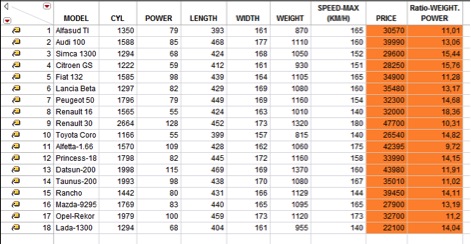
The data set has 18 rows with eight numerical columns. We could investigate relationships between pairs of variables. For example, maximum speed is correlated with power.

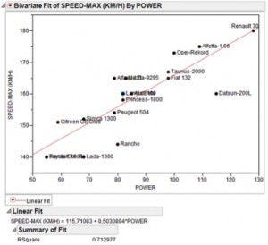
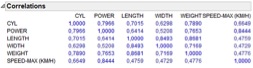
But with a large number of variables, it is more convenient to summarize the pairwise relationships with a correlation matrix, and we observe a large number of positive correlations. We also see that maximum speed is most strongly correlated with cylinder and power.

Because of the correlation structure in this set of variables, we can expect to reduce the number of dimensions using PCA.

We see that we have two distinct groups regarding the second component. One group is related to size characteristics of the car (length, width, weight), and the second group is related to motor characteristics (power, maximal speed, cylinder).

Illustrative Variables

Illustrative variables have no impact on the construction of the new components. They are used to help interpret the components and relate them to other variables (in this case, price and weight to power ratio).

You can download the JMP add-in for PCA with illustrative variables from the JMP File Exchange. (Download requires a free SAS profile.)

This add-in will allow you to add illustrative variables to a PCA .

Using our previous example, PCA with illustrative variables allows us to visualizethe relationship between the price and ratio of weight to power (orange variable in the previous data set) and the principal components without using these additional variables to build the PCA.

We can see that price is clearly correlated with all variables and grouped with the number of cylinders, power and speed-max. So an expensive car is a big car or a powerful car.

The second illustrative variable, the weight to power ratio, is negatively correlated with the power of the car regarding the two components and is negatively correlated with weight regarding the first component. It is clearly due to the fact that the weight can have negative impact on the power of a car.

References

G. SAPORTA, « Probabilités, Analyse de données et Statistique », TECHNIP, 2006 (in French).

Comments

WP_Comment

Joel Dobson wrote:

Suppose I have a semiconductor test program with 1000 datalogs. Each datalog is some electrical measurement on an IC chip and is a continuous variable. Each datalog might be a resistance, a current, a capacitance, an inductance, or a voltage, for instance, among other things.

One might have many voltages of the same type measured on each chip, corresponding to transistors of similar design but differing size for instance. These multiple readings may often have extensive multicolinearity among them. For example, threshold voltages are inherently related to drive currents and drive currents to leakage currents.

My goal is to see if I can reduce test time by only measuring the few datalog parameters that explain most of the variation, and stop measuring the ones that are highly multicolinear with those I keep reading.

I had thought of using PCA to reduce the dimensionality as you suggest, but each PC eigenvector is a linear combination of all the datalog parameters. So, although moving to the first few PCs does reduce dimensionality of the problem, but does not reduce my test time. Can you help me figure out how to do what I am trying to do using JMP 10? (I do not have JMP Pro.)

Regards, Joel Dobson

WP_Comment

Mike Clayton wrote:

Thanks very much. You can find perhaps more ideas including some datasets from earlier software efforts this important field. The Chemometrics and Control Systems people traditionally use Matlab and there is a toolkit for Matlab PLS which works with PCA to deal with many more complex multivariate problems. Eigenvector Research team taught MV methods at Sematech many years ago, and at that time the only tools in JMP were the Spin Plot and its subroutines. They used some of their quarry datasets to show us how to use that feature in JMP, as limited as it was. Another multivariate monitoring leader for many years was Svante Wold, who founded Umetrics. PCA when combined with PLS (can mean Partial Least Squares, or Project Latent Structures) can be used for MV SPC monitoring I am told (no personal experience doing that, however).

WP_Comment

Anish Nair wrote:

Madam do u know how find the accountability proportion from the principal components???

WP_Comment

Dan Obermiller wrote:

Joel,

Probably the best answer to your question is to use variable clustering (http://blogs.sas.com/content/jmp/2013/03/13/variable-clustering-in-jmp/ ). However, that is a JMP Pro feature.

With some effort and subjective opinions, you can use the loadings plot (the plot with a ray representing each variable) from PCA to reduce the number of variables that you measure. All of the rays that are pointing in approximately the same direction are highly correlated with each other. Therefore, you could just just one of the "set" to represent all of the variables in that set. This appraoch should help you reduce the number of tests that you need to perfrom.